A study of those factors that affect the propagation of sound energy in the sea and determine the
subsurface path of a sound beam after it is transmitted from a transducer is essential to a full
understanding of the sonar problem. Some of the
factors that make up the transmission anomaly
were discussed in chapter 1. The influence of
temperature conditions in the upper layers was
especially noted.
The variability in the transmission loss was first
observed in actual echo-ranging operations at sea.
In certain areas, the ranges achieved in the afternoons of clear, relatively calm days were found to
be less than those obtained in the mornings.
Temperature gradients change from season to
season, from day to day, and even from hour to
hour and place to place. Numerous explanations
were advanced, but the true reason was discovered
by the Woods Hole Oceanographic Institution as
the result of experiments performed in cooperation
with the Navy.
In many respects the ocean is very similar to
the atmosphere, and thus there is a close analogy
between oceanography, on the one hand, and
meteorology and climatology on the other. One
may speak of the subsurface weather and of its
seasonal and diurnal changes, of the subsurface
climate, and the annual and seasonal averages of
the components of the weather.
The analogy between oceanography and meteorology holds true further in that one of the practical
objectives of the oceanography of underwater
sound is the forecasting of subsurface weather.
The study of subsurface weather was neglected
until its importance for underwater acoustics was
recognized.
General Processes and Their Interaction
The outstanding characteristic of weather, both
in the air and under the sea, is its changeability.
This changeability is the outcome of a complex set
of processes, which are continuously in action.
Sometimes one of these processes may dominate
all others; more often, several exert appreciable
influences on the resultant.
There are at least 10 such processes that cause
the temperature gradients in the upper layers of
the ocean to change. They can be grouped conveniently into four general processes-(1) heating, (2) cooling, (3) mixing, and (4) flowing at a
speed different from that of the underlying water.
All four processes are closely interrelated but each
has its own characteristic effect on the temperature
gradients that are revealed by bathythermograms.
Each process is caused by a variety of factors.
All four, however, are affected by the condition of
the atmosphere at the ocean surface. The immediate effect of each process is to alter the dynamic state of the surface layers.
Table 2 presents an outline of the general processes, with their causes and dynamic effects. A
characteristic complication is illustrated by processes 2 and 3-cooling makes the surface layer
unstable, and instability in turn causes mixing.
In the same way, strong currents may cause turbulence, which again results in mixing. There
are many other chains of cause and effect linking
all the processes.
32
TABLE 2 -Outline of Processes Influencing Temperature
General process
Cause
Dynamic effect
Heating
Sunshine and/or warm, moist air.
Stability of surface layer.
Cooling
Evaporation, back radiation, and/or cold, dry wind.
Instability of surface layer.
Mixing
Wind and waves, instability and/or turbulence.
Neutral stability of surface layer.
Flowing
Wind and waves, internal waves, and/or currents.
Variable; turbulence if strong.
STRATIFICATION OF THE OCEAN
Bathythermograms show that the ocean is more
or less stratified. Two points separated by several
hundred yards but at the same depth beneath the
surface have practically the same temperature.
If the ocean were in equilibrium, this stratification
would be complete. The warm, lighter water
would be at the surface; the cooler, heavier water
would be at the bottom; and the boundaries between strata would be horizontal surfaces. Such
an equilibrium is disturbed by three of the four
general processes. The observed stratification is
thus the result of other processes tending to bring
the ocean to equilibrium.
DENSITY
It is a general hydrodynamic principle that when
a mass of fluid is in stable equilibrium under the
force of gravity its density must everywhere increase in the downward direction and be constant
in every horizontal plane. A commonplace illustration of this principle is furnished by a bottle containing oil and water.
The density of sea water is determined primarily
by its temperature and salinity. The changes due
to temperature are the largest, just as with the
velocity of sound. However, salinity has a proportionately greater effect on the density of sea
water than on the velocity of sound.
In the open ocean, where the salinity is practically constant, the lighter water almost always is
the warmer water, and it is to be expected that the
temperature either remains constant or decreases
with increasing depth. Near the shore, salinity
differences may sometimes dominate the density
distribution so that a layer of cold dilute water
may overlie warmer water of high salinity.
THERMAL STRUCTURE AND STABILITY
The concept of stability is a convenient one to
apply. Stability depends on the rate at which
density increases with depth. If the temperature
in a layer decreases rapidly with depth, as in the
thermocline, the layer has high stability, for the
density increases rapidly. On the other hand, a
layer in which the density decreases with depth is
unstable and exists only transiently.
Mixing processes are retarded by high stability;
thus wind of a given strength may easily mix a
surface layer in which the temperature gradient
is small and the stability is low. The same wind
may have little mixing effect if the temperature
gradients near the surface are large. The development of a sharp thermocline tends to retard mixing
to greater depths.
A completely mixed isothermal layer has neutral
stability. Cooling at the surface increases the
density of the surface layer, Evaporation, because
of the cooling and the increase in salinity that
accompany it, also increases the density of the
surface layer. Hence these processes tend to make
the density of the surface water greater than that
of water immediately below it and to produce a
condition of instability. This unstable density
distribution near the surface results in convective
mixing.
The stability can be estimated from a bathythermogram if the salinity gradients are assumed
to be negligible. Density decreases with increasing
temperature and for most practical purposes the
isotherms on the bathythermogram grid can be
interpreted as lines of equal density. The slope of
the temperature trace is therefore a measure of the
rate of change of density with depth-that is, of
stability. If this fact is kept in mind, the bathythermograph traces can be interpreted in terms of
the four major processes.
LABORATORY EXPERIMENTS ON
STRATIFICATION
Negative thermal gradients are very stable
because there is little exchange of heat between
neighboring layers unless they are mixed by some
General Processes and Their Interaction
33
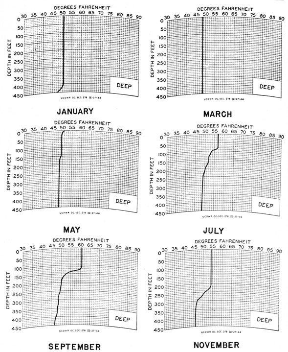
Figure 2-1 -Annual cycle of ocean temperature gradients.
34
stirring action. This fact is shown readily by laboratory experiments. If a tank is partly filled with
warm water, and if water of room temperature is
then run in through a hose lying on the bottom, the
warm water floats on the colder. Thermometers
placed in the two layers show that the cooler water
is not heated by the overlying warm water.
This stability of layers when the temperature
gradients are negative is in marked contrast to
the instability of positive temperature gradients.
In the experiment of warm and cold layers of water
in a tank, the surface of the warm layer may be
cooled by blowing a gentle stream of cold air over it.
The cooling of the layer at the immediate surface
causes it to become heavier than the water beneath
it. Consequently it sinks and in so doing mixes
with and cools the underlying water. Two thermometers at different depths in the warm layer
show that cooling proceeds nearly simultaneously
at all depths, without the development of large
positive temperature gradients. The mixing that
accompanies cooling is called convective overturn.
EFFECTS OF THE GENERAL PROCESSES ON
TEMPERATURE STRUCTURE
Heating
The progressive or intermittent effects of the
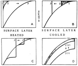
four processes-heating, cooling, mixing, and flowing-lead to the complicated and variable conditions illustrated in figure 2-1. The manner in
which any one of these processes operates individually to change the bathythermogram is shown
in figure 2-2. The change in temperature distribution produced by solar heating is illustrated
by curves 1, 2, and 3 in figure 2-2, A. Initial
conditions, indicated by curve 1, are assumed to
be isothermal. The absorption of heat, accompanied by some mixing, results in curve 2 and
finally curve 3. Negative gradients extending
from the surface downward are characteristic of
recent heating. The negative gradients, and consequently the stability, become greater as the
amount of mixing that occurs during the heating
becomes smaller. Under these conditions, wind is
the principal cause of mixing.
Cooling
The cooling that takes place during the night
and during the winter is essentially a reversal of
the heating process. In curve 1 (figure 2-2, B),
Figure 2-2 -Manner in which the general processes working
individually change the bathythermogram. A, development of negative gradient by heating of surface layer; B,
development of isothermal surface layer by cooling; C,
development of isothermal surface layer by mixing; D,
effect of current.
which is assumed to be the same as curve 3 in the
preceding diagram, surface cooling with its accompanying convective overturn produces curve 2
and ultimately curve 3. If continued long enough,
it would finally produce completely isothermal
water. Although the cooling takes place at the
surface, measurable positive gradients do not
develop because of the mixing involved in the
convective overturn. Winds hasten this mixing
process, but convective overturn takes place even
in very calm weather. Theoretically, the upward
transfer of heat must be associated with slight
positive gradients, but such gradients are so small
that they usually escape detection.
Mixing
The result of vigorous mixing by the wind, when
there is no gain or loss of heat by the surface layer,
is illustrated in figure 2-2, C. Note that in this
example surface isothermal layers develop just as
they did in figure 2-2, B, and the surface temperature decreases, but the temperature distribution
immediately below the mixed layer is different.
The wind mixes warm water with cooler water
beneath it, increasing the temperature at intermediate depths, and thus produces a very sharp
thermocline instead of retaining the initial gradients present when cooling is the primary cause of
the mixing. Curve 1 in figure 2-2, C, is the same
35
as curve 1 in figure 2-2, B, but the result of wind
mixing without cooling produces distributions
quite different from those resulting from cooling
alone. Obviously, conditions intermediate between those of figures 2-2, B, and 2-2, C, often
develop, because cooling and wind mixing can
occur simultaneously.
Flowing
The effect of addition or removal of water by
currents is illustrated in figure 2-2, D. Curves 1,
2, and 3 show the development of an isothermal
layer; curves (1), (2), and (3), of a negative
gradient. The transfer of water can be produced
by various causes, such as winds. If warm surface
water is carried over the top of cooler water, a
progressive change in temperature distribution
may occur, as illustrated by curves 1, 2, and 3.
If warm surface water is removed, the reverse
sequence, indicated by curves (1), (2), and (3),
may develop. Note that the gradients remain
unchanged and are merely lowered or raised.
Internal waves,. which periodically raise and lower
the thermocline, can cause similar effects in a very
short time. These waves may be single or have a
well-defined periodic character and are accompanied by single or periodic surges of current.
TEMPERATURE DISTRIBUTION
The four general processes all involve passage
of time-that is, continued heating, cooling, wind
mixing, or flowing produces progressive changes in
the temperature distribution. In the sea the
temperature distribution in a given locality is the
result of interplay of all four processes. For a
limited time, such as during one afternoon, one of
them may dominate, so that the temperature
conditions near the surface are the result of
heating, cooling, wind mixing, or currents. The
complicated distributions illustrated in figure 2-1
are usually the result of intermittent action of
the four general processes.
Thermal Structure at Great Depths
All these processes except the flowing originate
at the sea surface, and their effects are propagated
to greater depths by convective overturn or mixing
or both. These effects are rarely noticeable at
depths greater than from 600 to 700 feet. Below
these depths, stable stratification exists at all
times, and the only changes are due to slow
seasonal currents. This deep region is therefore
characterized by the so-called permanent thermocline or negative temperature gradient.
The density of sea water increases with decreasing temperature down to the freezing point (about
28.5° F), which sets a lower limit for the temperature in the sea. Below 6,000 feet the temperatures
everywhere are less than about 37.5° F and decrease with depth. They also decrease toward the
south, where the coldest water is formed.1 The
circulation of the deep, cold water is exceedingly
slow, probably of the order of 1 foot per minute.
For all practical purposes the conditions in the
deep sea do not change with time; they do, however, vary slightly from one region to another. In
any one locality below about 3,000 feet the temperature decreases slowly and the salinity is either
constant or increases slightly with depth.
Annual Cycle
In middle and higher latitudes there is a marked
annual cycle in temperature conditions. The cycle
can be observed in figure 2-1, which is based on
bathythermograms taken in the open ocean, in
latitude 40° N in the North Pacific.
It is convenient first to consider conditions in
March. The isothermal layer then is more than
450 feet thick, and is produced by cooling and by
mixing induced by winter storms. In May some
heating of the surface layers occurs, and mixing
by winds produces an upper isothermal layer of a
slightly higher temperature than the original;
thus, there is a small thermocline at a depth of
about 150 feet. The negative gradient at the
surface probably represents heating during the
day and is either obliterated by wind mixing or
disappears during the night because of cooling
and convective overturn.
Progressive heating continues through the summer months so that the temperature near the
surface increases, as shown by the July and
September bathythermograms; but wind maintains a mixed layer with a rather sharp thermocline, which increases in depth as the season
progresses.
1 H. U. Sverdrup, M. W. Johnson, and Richard H. Fleming, The Oceans,
New York, Prentice-Hall, 1942.
36
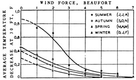
Figure 2-3. - Effect of wind on the average temperature gradient in the surface layer during various seasons.
In the fall, cooling once more exceeds heating;
the surface isothermal layer becomes cooler; and,
with the added effect of strong winds, the thermocline goes deeper until in January it is below 400
feet. Cooling and mixing continue until about
March.
In general the systematic seasonal changes are
subject to modification by local weather conditions.
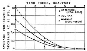
The mixing of the surface layer by wind is especially important in this connection. In figure 2-3
the average temperature decrease in the top 30
feet is plotted for each season as a function of
wind force. High winds can practically obliterate
the seasonal trend.
Diurnal Cycle
The diurnal cycle in temperature conditions is
in many ways a miniature replica of the annual
cycle, but it must be remembered that progressive
heating occurs during the spring and summer and
that progressive cooling and mixing occur during
the fall and winter. Consequently, the daily cycle
sometimes is practically obliterated by the progress of the seasonal changes.
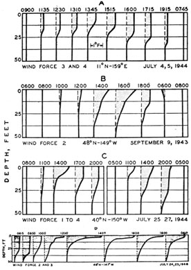
Four selected examples of diurnal changes are
given in figure 2-4. The data are from the open
ocean and are based on bathythermograms taken
over periods of from 23 to 48 hours during the
summer. Each set has been adjusted so that the
temperature at a depth of 50 feet is used as the
reference. The heating is indicated by shading.
The series shown in figure 2-4, A, was taken
during a day when winds averaged force 3. Although heat was added to the water, the stirring
action of the wind caused a mixed layer to persist
near the surface throughout the day. The layer
was so shallow, however, that poor sonar conditions prevailed during the afternoon. During the
night, cooling and mixing resulted in isothermal
conditions to a depth of 50 feet.
The series shown in figure 2-4, B, is an example
of heating on a day with light winds when negative
gradients extended to the surface during the late
morning and afternoon. Beginning at 1800, a
mixed layer was present and cooling continued
during the night. An observation at 0600 the next
morning showed a small positive gradient which
had disappeared by 0800.
The series shown in figure 2-4, C, covers a period
of approximately 48 hours with variable winds.
No progressive heating is noticeable, and there is
a return to isothermal conditions each night.
Figure 2-4 -Diurnal cycle of ocean temperature gradients.
A, Persistent mixed surface layer; B, typical diurnal cycle
with light winds; C, variable winds with changeable pattern;
D, persistent negative gradients.
37
The series shown in figure 2-4, D, is an example
of heating when a negative gradient existed early
in the morning. The shallow isothermal surface
layer had practically disappeared at noon; the
gradient became progressively more pronounced
during the day and persisted during the following
night.
As in the annual cycle, high winds can obliterate
the daily cycle in the upper 30 feet. This fact is
shown in figure 2-5.
Figure 2-5 -Effect of wind on the average temperature gradient
in a surface layer at various times of day.
Afternoon Effect
In general, strong negative surface gradients are
most common in the afternoon and produce what
is called the afternoon effect. The gradients reach
a maximum about 1600 and a minimum about
0600. Because solar radiation is greatest in the
summer, such gradients are more common during
the summer than during the winter.
This simple explanation is essentially correct
but fails to provide an explanation of the geographical distribution effect. Instead of being
most frequent at the equator, where solar radiation is greatest, the afternoon effect is actually less
frequent there than in high latitudes. Solar
radiation is undoubtedly the primary cause of the
negative surface gradients, but the magnitude of its
effect is modified by the other three factors,
especially wind mixing and evaporation.
Although in the open ocean, afternoon effect is
most frequent in high latitudes, this principle does
not necessarily apply inshore. The waters off
southern California, for example, are noted for
the prevalence of afternoon effect.
Analysis of the Four Processes
The preceding paragraphs have indicated the
general types of temperature distribution
encountered in the sea and the four major processes that affect the temperature conditions.
The causes of temperature conditions will now be
discussed.
HEATING AND COOLING
The temperature structure of the ocean is
determined primarily by its heat content, which
is a constantly varying quantity. There is a
continuous exchange of heat at the surface of the
ocean. The ocean receives heat by absorption of
the sun's radiation and by the condensation of
water vapor in the air when the water is colder
than the air. The ocean loses heat by radiation to
the sky, by evaporation of water vapor when the
water is warmer than the air, and possibly by
conduction. Of the received heat, by far the
largest quantity is due to incoming solar radiation.
Over the ocean as a whole incoming solar radiation
is balanced by the cooling resulting from reradiation and evaporation. The effects of other processes are comparatively negligible.
Incoming Radiation
The incoming radiation includes the invisible
infrared and ultraviolet as well as the visible
light. Because it is received from the sun and the
earth's atmosphere it obviously varies with latitude, time of the year, time of day, and atmospheric conditions-particularly the cloud cover.
The total energy received during the year decreases
with increasing latitude. In the lower latitudes
of the tropical regions the seasonal variation is
small, but with increasing latitude the difference
between the amounts received during the summer
and winter becomes very great. The effect of
clouds is very pronounced-a heavy cover of
cloud may reduce the incoming radiation to less
than 25 percent of that received on a clear day.
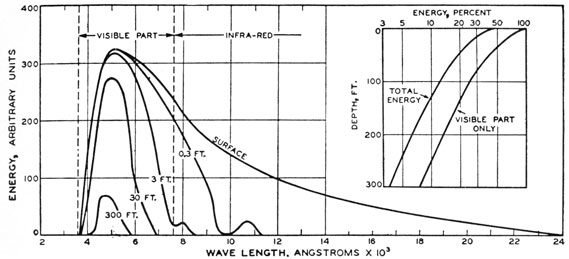
Direct heating of the water by the sun is limited
to relatively shallow depths (fig. 2-6). Only
about 3 percent of the radiation penetrates below
300 feet and over 50 percent (all of the infrared)
is absorbed in the first few inches. If there were
no compensating heat losses and no mixing,
fantastically high surface temperatures and extremely sharp negative gradients just below the
38
Figure 2-6. -Spectrum of radiant energy at various depths in the ocean. Insert: Percentage of incident radiation reaching various depths.
surface would occur. The penetration of light
varies somewhat from place to place depending on
the amount of suspended debris and organic pigments in the water. The foregoing discussion
applies to the open ocean. Near shore and in
areas of vigorous plant growth the water is practically opaque to all wavelengths.
Besides the direct solar radiation, the sea surface
also receives some infrared from the air. Although
the air is an appreciable source of heat, it is
customary to subtract it from the corresponding
infrared radiation emitted by the sea surface.
Effective Back Radiation
The excess of infrared emitted by the sea surface
over that received from the air is called effective
back radiation.2 Effective back radiation balances
somewhat less than one-half of the incoming solar
radiation, on the average. It decreases with increasing water temperature and with increasing
humidity and cloud cover. With heavy, low-lying
clouds present, the effective back radiation drops
to less than 25 percent of that on a clear day,
largely because the clouds are themselves sources
of infrared and radiate heat into the ocean on
their own account. Clouds prevent direct solar
radiation from reaching the sea surface. Heat
2Oceanography for Meteorologists. New York, Prentice-Hall, 1942.
losses from back radiation occur in the uppermost
fraction of an inch of the water and are transmitted
to greater depths by convective overturn and
wind mixing.
Evaporation
Evaporation depends primarily on the temperatures of the water and the air, on the humidity,
and on the wind strength. Evaporation can be
understood best by considering the process as one
of transfer of water vapor away from the surface.
The greater the water-vapor gradient, the more
rapid is the evaporation and hence the greater is
the heat loss. Cold, dry air overlying warm water
therefore favors rapid evaporation. High winds
increase evaporation by removing the water vapor.
The relative importance of the heat losses
through evaporation and back radiation can be
seen from the average heat budget between 70° S
and 70° N, as follows:
cal/cm2/min
Total heat received
0. 221
Evaporation losses
0. 118
Effective back radiation
0. 090
Conduction to atmosphere
0. 013
Total heat lost
0. 221
39
MIXING PROCESSES
Convective Overturn
Thus far only the cooling effect of evaporation
has been considered. When surface water cools,
its density increases and causes convective over-turn. Equally important is the increase in
salinity resulting from evaporation; the increased
density arising from this cause contributes greatly
to overturn and to the development of isothermal
surface layers. Thus, cooling by evaporation is
even less likely to be accompanied by positive
temperature gradients than is cooling by back
radiation.
Conditions that tend to lessen the salinity of
the surface layer would, of course, have the opposite effect and would tend to favor the development of positive gradients. Such a condition
might result from precipitation. For the ocean
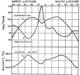
as a whole, however, evaporation exceeds precipitation. This fact is illustrated in figure 2-7.
Shaded areas show regions where precipitation
exceeds evaporation. The symbol 0/00 represents
parts per thousand. Note that regions of excess
evaporation in low latitudes and mid-latitudes
correspond to regions of relatively high surface
salinity and deep thermoclines. Just north of the
equator and in latitudes above 40°, where precipitation exceeds evaporation, the surface salinity
is low.
Figure 2-7 -Variation of average evaporation, precipitation,
and salinity with latitude.
Figure 2-8.-Effect of wind on the temperature gradient in the
surface layer at various latitudes.
The deficit in the water content of the ocean
that is caused by the general excess of evaporation
over precipitation is made up by run-off from land.
Near land-especially near the mouths of rivers-surface salinities are lower than in the open ocean.
This condition favors the development of positive
temperature gradients, because it increases their
stability.
Mechanical Mixing
Mechanical mixing is caused by wind and does
not necessarily involve any gain or loss of heat.
nevertheless, it may modify the temperature
distribution. The effect of winds depends not
only on their strength, but also on their duration
and on the distance over which they have blown
It is obvious that the first effect of the wind is
confined to the immediate surface, but that the
turbulence extends to greater depths after the
wind has been blowing for some time. The
original density distribution of the surface layer
affects the rate at which the turbulence penetrates
the layer. A very stable layer is less easily mixed.
Effect of Rotation of the Earth
The daily rotation of the earth about its axis
also affects the depth to which the wind mixing
penetrates. Present theories agree that a wind of
given force ultimately produces a deeper mixed
layer in low latitudes than in high.
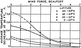
This principle is probably part of the explanation
of the data shown in figure 2-8, which indicate
that strong negative gradients are most apt to be
formed in high latitudes. If negative surface
gradients are interpreted naively as being the
result of solar heating alone this condition is most
40
unexpected, because heating is greatest at the
equator. The necessity for considering all four
of the major processes, with the detailed mechanisms causing them, is emphasized by figure 2-8.
CURRENTS
Drift Currents
The frictional drag of the wind sets up drift
currents which flow at less than 3 percent of the
wind velocity. These drift currents do not
flow with the wind, but are deflected 45° to the
right in the Northern Hemisphere and 45° to the
left in the Southern Hemisphere. This deflection
is caused by the earth's rotation and is closely
related to the influence of the earth's rotation on
the depth of mixing, which was just discussed.
Permanent Currents
The redistribution of density resulting from the
wind-drift currents in turn maintains the permanent currents. Under the influence of the steady
wind systems, such as the trade winds in the low
latitudes and the westerlies in high latitudes, these
permanent currents form the large-scale current
system of the oceans. They are thus partly the
indirect result of geographic differences in the
heating and cooling of the water and partly the
result of wind action. The character of the
currents is influenced also by the configuration of
the oceans, but in general there are clockwise
gyrals in the Northern Hemisphere and counter-clockwise gyrals in the Southern Hemisphere.
Smaller currents related to land topography and
local climate exist near the continents. A counter
current flows eastward between the two westward-flowing equatorial currents.
The permanent currents have several effects on
the temperature conditions. Currents with poleward flow tend to carry warm water into cooler
regions. Conversely, currents with equatorward
flow tend to carry cool water into warmer regions.
Within the currents themselves the distribution of
density produces a temperature gradient such
that in the Northern Hemisphere the water on
the left side of the current has a lower average
temperature than the water on the right side.
This condition may be reflected by a thinner
mixed layer or even by lower surface temperatures.
In the Southern Hemisphere the structure is
reversed.
Divergence and Convergence of Surface Currents
Divergence of the surface currents may occur
under the influence of the wind. Examples of
this effect are found along the western coasts of
the continents and in the vicinity of the equator
in the eastern parts of the Atlantic and Pacific.
In these areas upwelling brings water toward the
surface from moderate depths and the thermocline
may be shallow or, rarely, absent.
The opposite effect, convergence, occurs in the
center of the subtropical gyrals in the Northern
and Southern Hemispheres. In these regions the
surface water accumulates, and consequently the
thermocline may be very deep.
Tidal Currents
Tidal currents in partially isolated, shallow
areas have a marked effect on temperature conditions because they also cause turbulent mixing.
In areas of strong tidal currents-for example in
the English Channel-the water may remain
virtually mixed throughout the year, although
there is heating and cooling of the water column
as a whole.
Internal Waves
Internal waves also affect the temperature distribution. The effect of these waves is reflected
in a periodic rise and fall of the thermocline.
Periods as long as 24 hours are known to exist,
and recent studies have shown that periods of
only a few minutes may occur. Whether there is
a continuous spectrum of frequencies is not known.
Geographical Variations
DEPENDENCE OF THE ANNUAL CYCLE ON
GEOGRAPHICAL LOCATION
The annual cycle in temperature conditions
represents the net effect of the annual sequence in
the various factors described, particularly in the
amount of radiation received, the heat losses
associated with evaporation, and the character of
prevailing winds. In low latitudes where these
factors do not vary appreciably there is little
41
change in conditions throughout the year, except that near the continental
boundaries changing
monsoon winds may introduce variable conditions.
The annual cycle is most conspicuous in the latitudes of from 40° to 50°.
This condition is to be
expected, because in these regions the surface experiences the greatest
range of temperature.
The effects of this great variation in temperature are magnified by the
fact that in winter the
cooling due to low temperatures is increased by the greater evaporation
that occurs at this
season. The resultant increase in the density of the surface water
facilitates mixing and thus
contributes to the seasonal variation.
The annual cycle is even more pronounced in regions near land, and in areas
where heavy
precipitation occurs and light winds prevail during the spring and summer.
These conditions
tend to induce even more extreme negative gradients than those shown in
figure 2-2. These
gradients can also be observed generally in areas of flow toward the
equator, in which cool
water is being heated-for example, off the California coast.
DEPENDENCE OF THE DIURNAL CYCLE ON GEOGRAPHICAL LOCATION
The diurnal change in temperature gradients is essentially similar in
principle to the annual
cycle, but the temperature changes are smaller and do not extend to such
great depths. The
incoming
solar radiation depends on latitude, time of year, time of day, and
cloudiness. The diurnal cycle
of incoming radiation changes during the year, the variation being least
near the equator and
increasing toward the poles. Above the polar circles, of course, there are
days of complete
darkness during winter and continuous daylight during summer. The diurnal
change is not
necessarily cyclic, as is time annual change, and progressive heating or
cooling of the water is
characteristic in middle and high latitudes. Within the tropics, where the
annual variation is
small, diurnal changes are more nearly cyclic.
Even if the total heat absorption is the same, the character of the changes
in temperature
gradients may be quite different, because these changes depend on the
previously existing
gradients and on the wind conditions. A negative gradient near the surface
is increased by
incoming heat unless a strong wind (force 4 or greater) springs up. On time
other hand, the
changes in an initially mixed (isothermal) layer depend critically on the
wind strength. The
development of surface gradients is common when the wind force is 3 or less
but is rare with
winds above force 4. (See figures 2-3, 2-5, and 2-8.) In the trade-wind
belts, therefore,
development of surface gradients during the day is a rather rare
condition-probably another
factor to be considered in explaining figure 2-8.
Summary of Conditions for Temperature Gradients
The regional differences in temperature structure can be explained in terms
of the factors
described. The discussion can be summed up as follows:
An isothermal layer near the surface is the result of mixing. The factors
inducing mixing are
(1) wind, (2) radiative cooling, (3) evaporation, with its consequent
cooling and salinity
increase.
Strong negative gradients are the effect of heating a stable surface layer,
without much wind
mixing.
Strong winds may tend to prevent the formation of negative gradients.
Positive gradients are produced only in areas where cool, dilute water
flows or is formed on top
of warm, more saline water. Measurable positive temperature gradients are
most common
during the fall and winter months in the northwestern Atlantic and Pacific
Oceans, where cold,
dilute coastal waters are driven offshore by the wind and flow over the
warm. but saline ocean
water of higher density.
Wakes
Echo formation from discontinuities in a
medium, such as suspended air bubbles in water, has been discussed in
chapter 1. In sonar, the
principal source of discontinuities that produce
echoes, reverberation, or scattering is the wake of
a ship. The acoustic properties of a wake are important because of their
influence on
transmission and operational procedures.
42
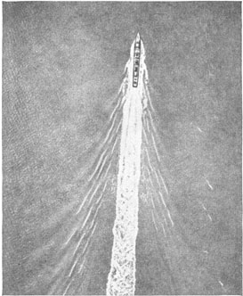
Figure 2-9. -Wake of U. S. S. Moole (DD) at 20 knots, From 2,500 Feet.
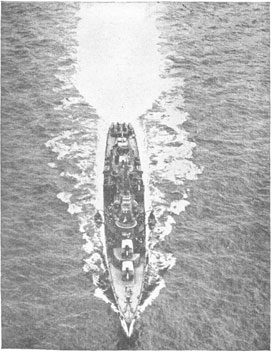
Figure 2-10. -Woke of U. S. S. Ringgold (DD) from 300 feet.
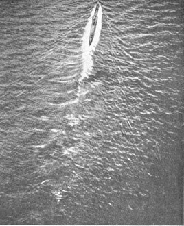
Figure 2-11. -Wake of surfaced submarine at 15 knots.
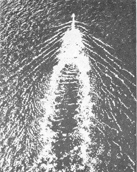
Figure 2-12. -Swirl behind submarine after crash dive.
43
VISUAL APPEARANCE
The wake of a ship is most readily seen from the
air (figures 2-9 through 2-12). The surface waves
that spread out in a V-shape behind the vessel and
form a navigational hazard for nearby small craft
are relatively inconspicuous from the air. Even
the white bow wave, which breaks and sends foam
back along the sides of the vessel, is inconspicuous
compared to the wake of the turbulent, foamy
water that fans out from the screws.
This turbulent wake spreads rapidly for a
fraction of the ship's length, and thereafter widens
only slightly. The divergence has been measured
for various wakes and found to vary from 0.5° to
5°. The foam, which makes it visible from a
distance, gradually disappears, but not until long
after the ship has passed. The visible wake of
a high-speed vessel extends from 20 to as much as
50 ship lengths astern.
PHYSICAL PROPERTIES OF WAKES OF
SURFACE VESSELS
It is fairly obvious that the violent disturbance
which creates the turbulent wake gives it physical
properties that differ to a greater or lesser extent
from those of the undisturbed ocean surrounding
it. For example, if there is a temperature gradient
in the upper part of the ocean, the mixing of the
surface water with that of lower layers gives the
water in the wake a different temperature from
that of the nearby water at the same depth. This
effect has been observed by the use of sensitive
recording thermometers. The mixing of water
from different depths may also result in anomalous
density gradients.
ACOUSTIC PROPERTIES OF WAKES
Of most interest at this point are the acoustic
properties of the wake. They are probably all
associated with the presence of entrained air
bubbles. Aerial photographs show, that large
numbers of bubbles remain in the wake for several
minutes. It is likely that some remain suspended
in the water even after the visible foam disappears.
These acoustic properties of the wake are easily
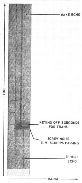
demonstrated with sonar gear. Figure 2-13 shows
a record of echoes obtained from the wake of the
E. W. Scripps. This vessel ran between the echo-ranging vessel and a small sphere, the echoes from
the small sphere being recorded simultaneously
with those from the wake.
Two general conclusions can be drawn from
figure 2-13o(1) the wake echo gradually lengthens
and becomes fainter, presumably because of the
spreading of the turbulent wake and the gradual
disappearance of the bubbles, and (2) the sphere
Figure 2-13 -Range recorder trace of wake echoes.
44
echo is weakened slightly but noticeably by the
wake between the sonar and the sphere.
Thus, we may conclude that the wakes of surface
vessels have two major acoustic properties-(1) they return echoes that are readily detectable
by ordinary sonar gear, and (2) they act as acoustic
screens, reducing the intensity of the echoes from
targets on the far side of the wake.
Causes of Acoustic Properties of Wakes
The two most obvious differences between a
surface wake and the undisturbed ocean are
(1) the turbulence of the wake and (2) its content
of bubbles. It is therefore reasonable to assume
that one or both of these factors are the cause of
its acoustic properties.
The possibility that turbulence is the cause of
wake echoes is ruled out by theoretical considerations. It is true that when a sound wave passes
through turbulent water it is scattered, but two
facts exclude the possibility that this scattering is
the cause of echoes-(1) the scattering from
turbulence is very weak unless there are great
differences in velocity between pairs of points
separated by 1 wavelength of the sound, and
(2) the intensity of the scattered sound depends
strongly on the direction of scattering, and the
intensity in the backward direction is zero. Thus,
although turbulent water scatters sound, it does
not return an echo.
Turbulence may be an indirect cause of the
echoes by mixing the warmer surface water with
that from below. From this mixing, irregular
differences of temperature are produced, which
cause irregular differences in sound velocity in the
turbulent water. However, the magnitude of the
expected effect is too small. To produce the observed echoes, temperature differences of nearly
1° F would have to occur between points only 1
wavelength apart. Such large temperature differences are very improbable. Moreover, if they
were formed in some way, they would persist for
a much longer time than wakes are observed to
persist.
Thus, it may be concluded that the air bubbles
in a wake are the major cause of the acoustic
properties of the wake. Several objections have
been urged against this conclusion. One objection
is based on the supposed short life of bubbles in
water. Bubbles rise to the surface and break, so
239276°-53-4
that they disappear from the wake in a short
time; their disappearance is also hastened by absorption of air by the sea water. On the other
hand, echoes have been obtained from wakes more
than 10 minutes after the vessel has passed, and
there have been reports of echoes from wakes
several hours old. The latter reports may be discounted, because it is very difficult to be certain
of the position of a wake so long after the ship
has passed, and it is quite possible that a school
of fish, for example, might be mistaken for a wake
under such circumstances. It is therefore necessary only to show that some bubbles remain suspended for periods of from 10 to 30 minutes.
Experimental evidence on this point was obtained by stirring the water of the pool at U. S.
Naval Electronics Laboratory (USNEL) with an
outboard motor. The acoustic properties of the
water were studied with an echo sounder. It was
found that sound was returned from the body of
the water after stopping the motor. This return
continued even after all the more obvious bubbles
and turbulence had disappeared. Closer examination showed, however, that a relatively small
number of small bubbles remained suspended.
They were very difficult to see except when they
drifted into a region of favorable illumination, so
that neither their number nor their size could be
accurately determined. It was concluded that
sufficient bubbles were present to explain the observed effects. This conclusion was based on the
consideration that very small bubbles are quite
effective in scattering sound and rise very slowly.
The rate of rise of the bubbles which are most
effective in scattering is about 1 yard per minute. These results for still water do not apply
directly. to wakes or turbulent water. The long-lived bubbles observed in the USNEL pool did
not show any marked tendency to rise but were
carried in irregular paths by the motion of the
water. This condition is analogous to the effect
of air currents in keeping dust from settling. It
is reasonable to suppose that the moderate turbulence in an old wake has this same effect and prevents the disappearance of the bubbles.
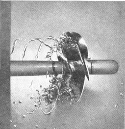
Propeller Cavitation as a Source of Bubbles
The second objection to air bubbles as the cause
of acoustic properties in wakes is based on the
fact that echoes are obtained from the wakes of
45
Figure 2-14 -Cavitating propeller.
submerged submarines and the idea that most of
the bubbles in a wake come from the breaking
bow wave. Aerial photographs strongly suggest
that, this idea is not correct, because most of the
foam appears to come directly from the screws.
This idea is borne out by the observation that the
wake laid by a vessel under sail is less acoustically
active than the wake of the same vessel under
power.
Hence, most of the bubbles are caused probably
by cavitation at the propellers. Photographs of
this phenomenon are shown in figures 2-14 and
2-15. In figure 2-14, the water in the jet is
moving away from the observer. The back of
each blade is half covered with cavitation bubbles
and a cavitation void which extends for some
distance behind the blade, whereas the face of
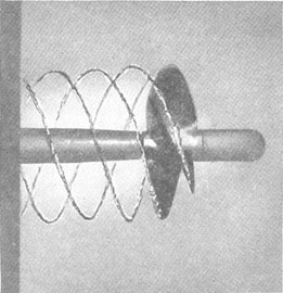
each blade is clean. In figure 2-15, the cavitation of the rotation of the propeller and the
flow of the water in the jet from left to right
gives a spiral pattern to the vortices.
The bubbles are formed far from the air-water
interface and are not sucked under from the
atmosphere. The mechanism of cavitation is
apparently similar to that of boiling. Because
of the motion of the screws the hydrostatic
pressure is reduced; the boiling point of water is
lowered by this reduced pressure and boiling
occurs. For example, pure water boils at 60° F
if the pressure is reduced much below one-sixtieth
of an atmosphere.
However, sea water is not pure. In the present
discussion, dissolved air is the most important
impurity. Dissolved air is present in such quantities that sea water boils at 60° F whenever the
pressure is reduced much below 1 atmosphere.
The bubbles produced by this boiling are filled
principally with air, rather than water vapor.
Once formed, these bubbles are apparently quite
stable-that is, the rate at which the air is
redissolved is very slow.
Even in the wakes of surface vessels, much of
the foam is probably the result of cavitation, and
only a part of it is probably caused by air dragged
under from the atmosphere. In the wakes of
submerged submarines the only sources of air
other than cavitation might conceivably be leaky
high-pressure air lines.
Dependence of Cavitation on Depth and Speed
Cavitation depends critically on propeller rpm.
A given propeller at a given depth of submergence
produces no bubbles unless its speed exceeds a
certain critical value; when the speed exceeds
No, the number of bubbles formed increases very
rapidly, but not according to any known law.
The critical speed itself, however, depends in a
simple manner on h, the depth of the propeller beneath the sea surface. Expressed as an equation,
this dependence is
No2/h = constant. (2-1)
Figure 2-15 -Tip vortices emanating From a propeller.
46
Thus, if a given propeller begins to cavitate at 50
rpm when at a depth of 15 feet, it begins to cavitate at 100 rpm when at a depth of 60 feet and at
200 rpm when at a depth of 240 feet.
The constant in equation (2-1) depends on the
design of the propeller, and on any accidental
changes in its shape that may occur in service. A
scratch or nick caused by some accident usually
reduces appreciably the value of the critical speed.
One remarkable property of cavitation is that the
bubbles themselves scratch and scar the metal surface on which they are formed.
This theory of the relation between cavitation
and the acoustic properties of wakes has certain
consequences that can be qualitatively checked.
Thus, the wake of a submerged submarine should
return echoes, but the echoes should be considerably weaker than when the ship is moving on the
surface. They should also become progressively
weaker as the depth of submergence increases.
Finally, they should increase rapidly with propeller
speed. All these conclusions are in general agreement with experience.
The propellers are probably not the only source
of cavitation bubbles. Because the ship as a whole
is moving through the water, cavitation can occur
at other places. In general, the smaller the object,
the lower is the critical speed at which cavitation
occurs. Thus, small fittings or handrails on the
deck of a submarine may become sources of cavitation bubbles when submerged.
PROPAGATION OF SOUND IN WATER
CONTAINING BUBBLES
The theoretical discussion of the acoustic properties of water containing air bubbles is complicated, and the studies are not complete. To present the general ideas of the theory without confusion, it is convenient to introduce certain terms for
the description of water containing bubbles.
In foamy water the average distance between
neighboring bubbles is less than the average diameter of the bubbles. The walls separating the
bubbles may occasionally be very thin, as with
soap suds. The acoustic theory of foamy water
has not been studied, but lack of this information
is not important because wakes probably contain
foamy water only at the air-water surface, where
the bubbles tend to accumulate.
In bubbly water the average distance between
neighboring bubbles is considerably greater than
the average diameter of the bubbles but much less
than the wavelength of the sound involved. For
practical purposes, water may be considered to be
bubbly if it contains less than 1 part per 1,000 (by
volume) of air and foamy if it contains much more
than this amount. The bubbles are dispersed if
the average distance between neighbors is greater
than both 1 wavelength of the sound and the average diameter. Thus, a portion of a wake may be
dispersed for ultrasonic frequencies and bubbly for
sonic frequencies.
It would be useful to have information concerning
the foamy, bubbly, and dispersed regions of typical
wakes. Unfortunately, there is relatively little
information of this sort other than that which can
be obtained from the inspection of aerial photographs or deduced indirectly from acoustic measurements. The wake probably reaches the dispersed state between 5 and 10 ship lengths astern
of the screws; it is foamy only in the immediate
neighborhood of the screws or at the air-water
surface.
Scattering and Absorption of Sound in Wakes
Except for some details, the theory of dispersed
wakes is similar to the theory of reverberation.
Consider a region where the acoustic energy of
a sound beam is flowing into a dispersed wake.
The bubbles remove power from the beam at a
rate that depends upon the intensity of the sound
in the beam and the total effective cross section of
the bubbles. Of the power removed from the
beam, a fraction is reradiated as sound. The
quantity of energy reradiated is determined by a
factor called the scattering cross section of the
bubbles.
The remainder of the power that is removed
from the beam is converted into heat-that is,
absorbed by the air of the bubbles and, to a lesser
extent, by the water surrounding them. The
quantity of energy converted into heat is determined by the absorption cross section of the bubbles.
Thus the total effective cross section is a combination of scattering and absorption cross sections.
Note that the total effective cross section determines the screening effect caused by a wake,
whereas the strength of the wake echo is determined by the scattering cross section.
47
Interpretation of Scattering Experiments
Historically the study of scattering and absorption has played an important part in the development of various branches of physics. This
development is especially evident in those branches
dealing with radiations that are not perceptible
by the unaided human senses-such as X-rays;
α rays; β rays; γ rays; cosmic rays; and more
recently, neutron rays. The scattering of visible
light explains the color of the clear sky and other
meteorological phenomena. The scattering of
sound waves had not been studied in any systematic manner before World War II. During the
war such studies were begun and are still far from
complete.
The modern knowledge of the structure of
matter, atoms, and nuclei is based largely on
scattering experiments. Experiments on the scattering of sound and radio waves are unlikely to
contribute much to this fundamental knowledge
concerning the imperceptible structure of matter.
Such experiments almost certainly will contribute
much to the knowledge of the inaccessible parts of
the ocean and the atmosphere. Thus studies of
reverberation and of the scattering of sound by
wakes are considered to be very important, even
apart from immediate practical objectives.
The interpretation of the experiments has been
the subject of much careful thought, and has
resulted in many major advances in knowledge.
However, examples of misinterpretations by conscientious and able experimenters are also
numerous.
The most common error is the measurement of
extraneous radiation along with radiation that is
intended to be measured. In measuring the intensity of sound transmitted through a wake, it
is most important to shield the hydrophone from
all sound that passes beneath the wake.
The interpretation of many laboratory experiments has been simplified by the use of opaque
screens to shield the detector from extraneous
radiation. Sometimes these screens have not
been completely opaque. Often their edges have
been the source of scattered radiation. In performing scattering experiments at sea, it is not
possible to use such screens, so that the probability
of extraneous sound is particularly great.
Another error is the application of theoretical
equations to circumstances that do not conform
to the assumptions made in deriving them.
TRANSMISSION OF SOUND THROUGH
WAKES OF SURFACE VESSELS
A series of experiments on the wakes of destroyers and destroyer escorts was performed by
the University of California, Division of War
Research (UCDWR).3 The procedure was as
follows: One vessel carried a hydrophone and was
dead in the water, while a destroyer ran past it
on a straight course at a fixed speed. As soon as
the destroyer had passed, a small launch got
underway and carried the sound source from one
side of the wake to the other. In this way it
was possible to measure the intensity of the sound
both when the wake intervened between source
and receiver and when the source was on the same
side of the wake as the receiver. After allowance
was made for the difference in range when the source
was on one side or the other of the wake, the apparent transmission loss caused by the wake was
determined.
It is not certain that the result is free from error.
In the first place, when the sound soured is on the
far side of the wake, it is possible that some sound
may pass under the wake and reach the hydrophone. This error was minimized by suspending
both source and hydrophone about one-half the
depth of the wake. In spite of this precaution,
it must be emphasized that the values of transmission loss so obtained are possibly too low.
This source of error can be eliminated by making
the measurement while the source is in the wake,
but in that case the value obtained may be too
large because of the effect of bubbles in reducing
the output of the source. To some extent this
value is counterbalanced because only part of the
wake is between the source and the receiver. The
true value probably lies between the two measured
values.
WAKE STRENGTH
Dependence on Age of Wake
Early experiments were performed with a single
vessel, the U. S. S. Jasper, which ran on a straight
3Sound Transmission Through Destroyer Wakes, OEMsr-30, Service Project NS-141, Report M-189, UCDWR, March 8, 1944.
48
course, then circled and echo-ranged on its own
wake.4 These experiments showed that the level
of the echo decreased fairly rapidly with the age of
the wake. The results of various experiments
ranged from 1.5 db per minute to 8 db per minute,
with an average of about 4 db per minute. The
levels of the echoes were compared with those of
reverberation on the same day at the same range
from the sonar. On one day this range was about
235 feet and the echoes were about 40 db higher
than either volume or surface reverberation.
These two kinds of reverberation were about equal
at this range. On another occasion the range was
140 feet and the echo was 17 db higher than surface
reverberation. A sea state 2 and wind force 3
prevailed on this occasion.
In view of the variability of reverberation from
day to day, these observations have little absolute
significance but serve to give some idea of the
strength of echoes from the wake of a small
slow-speed vessel. The values obtained for the
rate of decrease of the wake echo have greater
claim to validity and are in good agreement with
other observations.
The difficulties inherent in performing experiments on wakes at sea led to an extended series
of experiments in San Diego Harbor. A 40-foot
motor launch was used to lay the wakes, which
extended from the surface to a depth of about
5 yards.5 There was some evidence that sound
reflected from the bottom increased the strength
of the echo. To minimize this effect, only echoes
obtained at ranges of less than 100 yards are
included in the following averages.
TABLE 3. -Dependence of Wake Strength on Age of Wake
Frequency (kc)
Time of maximum echo (sec)
Wake strength at time of maximum echo (db)
15
30
-2.9
24
50
+3.1
30
70
+8.4
Echoes were obtained by using 15-kc, 24-kc, and
30-kc sound. These echoes did not reach their
4 Carl F. Eckart, Echoes from Wakes, NDRC C4-sr30-498. UCDWR,
August 29, 1942.
5 Richard R. Carhart and George E. Duvall, Acoustic Measurements of
Surface Wakes in San Diego Harbor, OSRD 1628, NDRC 6.1-sr 30-961, Report U-62. UCDWR, May 8, 1943.
Figure 2-16 -Variation of the wake echo level with age of the
wake, for various ping lengths at 24 kc.
maximum values until some time after the passage
A the launch through the sound beam. Average
values of the time of the maximum echo are shown
in the second column of table 3. Thereafter, the
echo intensity diminished at an average rate of
about 7 db per minute for all three frequencies.
The wake strength at the time of the maximum
echo level was computed for each experiment, and
average values are shown in the third column of
table 3.
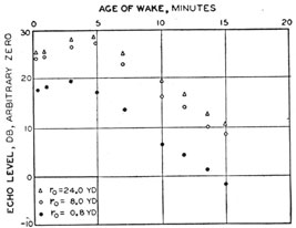
Figure 2-16 gives further information concerning
the behavior of wake echoes. The early period,
during which the echo from the wake increases
in level, is clearly evident, as is the later period
during which the echo level decreases at a rate
of about 1.8 db per minute.
Dependence on Ping Length
Figure 2-16 also brings out a dependence of
echo level on ping length. The theoretical
discussion has emphasized the analogy between
wake echoes and reverberation. Essentially the
wake is a part of the ocean from which the reverberation is especially high. If the ping length is
shorter than the width of the wake the distinction
between reverberation and wake echoes disappears.
The number of scatterers returning echoes at any
moment is determined, not by the extent of the
wake but by the ping length.
Wake Strengths of Submarines
Many difficulties are encountered in experiments
on the wakes of submerged submarines. The problems of navigation and seamanship involved in the
49
maneuvers are not always solved successfully, even
by the ablest submariners. These practical difficulties and the low levels of the wake echoes account for the conflicting reports that have been
made on the subject.
On one occasion echoes from the wake of an
S-type submarine were recorded with standard
echo-ranging gear operated at 24 kc. When this
submarine was running at a depth of 45 feet, contact was maintained with the wake at a distance
of 3,000 feet astern of the screws. At depths of 90
and 125 feet, the lengths of the contacts were 700
and 300 feet, respectively.
On a second occasion, an attempt was made to
use a recording echo sounder for the study. This
instrument had been successfully used in the study
of the wakes of surface vessels. Consequently, it
was mounted on a launch, and the fleet-type submarine ran on a straight course designed to carry
it directly under the launch. This maneuver
proved difficult to execute, but echoes from the
hull of the submarine were obtained several times.
The depth of the submarine varied from 65 to 200
feet. Echoes from the wake were never obtained
at distances more than from 50 to 100 feet astern
of the screws.
It had been hoped that this experiment would
show whether the wake has a tendency to rise to
the surface, as might be expected if bubbles are
the primary cause of its acoustic activity. The
results are inconclusive. It has been reported
that, on several occasions, the wake of a submarine
running at a depth of from 45 to 60 feet could be
seen from the deck of a nearby surface vessel. This
visibility was apparently due more to turbulence,
which disturbed the surface, than to bubbles.
On a third occasion, 15 experiments were performed to measure the wake strength of a fleet-type submarine running at various depths of from
45 to 400 feet. None of these experiments yielded
echoes that were positively identified as caused by
the wake, although echoes from the hull of the
vessel were obtained. Some few echoes may have
come from a short distance astern of the screws.
Frequencies of 20 kc and 45 kc were used; 45-kc
echoes from the wake would have been recorded
provided they were not more than 14 db below
those from the submarine itself. At 20 kc, the
echoes from the wake would have been recorded
provided they were not more than 28 db below
those from the submarine itself.
The operational problems were reduced to manageable proportions by the following procedure:
The submarine started on the surface, running a
course parallel to that of the echo-ranging vessel.
The echo-ranging vessel ran at a slow speed, so
that the submarine overtook it and passed through
the sound beam while still on the surface and at
a range of from 100 to 300 yards. About 90
seconds after passage the submarine dived rapidly
to 90 feet and slowed down. Simultaneously the
surface vessel increased speed and overtook the
submerged submarine about 10 minutes later. It
was found that these operations could be carried
out satisfactorily except that it was difficult to
adhere to the prearranged time schedule and that
the submarine's submerged course often diverged
appreciably from the course of the surface vessel.
The timing of events was critical because of the
limited supply of film in the magazine of the
recording oscillograph.
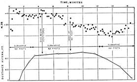
Data recorded during such an experiment are
summarized in figure 2-17. The lower half of the
Figure 2-17 -Wake strength of a submarine.
figure shows the distance astern in feet. Note
that the wake strength while the submarine was
running on the surface was from -10 to -15 db.
This wake strength was momentarily increased
as the echo-ranging vessel passed the site of the
dive, where the venting of air from the ballast
tanks presumably increased the bubble content
of the wake. After the submarine reached the
depth of 90 feet the wake strength varied between
-20 and -30 db, even while the distance astern
remained practically constant at about 900 feet.
50
TABLE 4 -Wake Strengths of Submarines
Submarine type
Frequency (kc)
Wake strength surfaced, 9 knots (db)
Wake strength submerged 6 knots (db)
Depth (ft)
S
60
-18
-26
90
S
45
-13
-24
90
Fleet
45
-13
-20
90
S
45
-33
45
S
20
-20
45
As the echo-ranging vessel overtook the submarine
the wake strength again increased to -20 db.
The results of other experiments with submarines
are listed in table 4. Ping lengths of from 8 to 24
yards were used in all the work summarized.
Even when the submarine is running on the surface, the strength of its wake is very small. This
fact can probably be explained by the low speeds
at which the submarine moves.